PhaseFlow, Open-Pit Production Schedule with a Certified Bound
An open-pit production schedule, solved with a certified bound and animated year by year over the block model. PitForge answers which blocks are worth mining; PhaseFlow answers when, subject to slope precedence in every period and per-period mining and processing capacity, maximising discounted NPV. That is the constrained pit limit problem (CPIT). The trust anchor is the published MineLib newman1.cpit solved AS PUBLISHED, on its own six periods, its own eight percent discount rate and its own two capacities: it reproduces the ultimate pit optimum exactly (26,086,899), its joint LP bound sits at 24,486,184, below the 24,486,549 LP bound published for the richer PCPSP problem, and its best schedule is 1.37 percent below that bound and 0.11 percent below an external integer optimum. The bound needs no LP solver (critical multiplier algorithm, exact in O(mn log n) as parametric maximum closures), which is why the whole problem re-solves live in the browser. Two bounds run on every case and the difference between them is reported, because that difference is the part of a gap that belongs to the bound rather than to the plan.
Business Context
A production schedule is where a mine plan turns into money and into commitments: it sets the NPV the project is valued on, the equipment fleet that has to exist each year, and the feed the plant will actually see. The value of a certified bound is that it converts a number into a statement with a limit attached, so the discussion moves from whether an NPV is believable to how much value is provably still on the table. Reporting both bounds is the same discipline applied one level deeper: it tells you whether the remaining gap is a weakness in the plan or slack in the mathematics used to measure it. Spatial coherence matters for the same practical reason: a schedule that scatters a period into many small components is expensive or impossible to actually mine, and the app reports components per period, largest-component share and the narrowest mined run as first-class KPIs rather than leaving mineability to a reviewer eyeballing a picture.
Strategic Value
PhaseFlow is the scheduling step of the open-pit line, and it earns trust by being measurable against work that is not its own. It solves a published MineLib instance as published and puts its numbers beside the published ones, and says which bound each gap is measured against. It computes its bound without an LP solver, which is what makes a genuine live lane possible rather than a replay. It runs two bounds on every case and reports their difference, so a gap can be attributed to the plan or to the bound. It treats spatial coherence as a KPI because the algorithm authors themselves predict block-level schedules scatter. And its learned lane is characterised rather than only measured: the answer to when the surrogate fails changed twice under measurement. The orebody first, then the discount rate on the held-out deposits, until a third split gave that rule a recall of 0.625 and exposed the study itself, whose sweep moved the discount rate and the plant capacity together (correlation -0.735). On a crossed sweep the signal is the orebody on both splits: two thirds of the core-and-halo cases fail and the layered ones never do. The product measures instead of predicting: every baked case carries the exact plan the learned rung approximates, and the ratio between them sits next to the method selector. On the live lane no usable guard exists yet, because a real deposit has no archetype label and the scenario rule catches only 0.44 of the failures, and the product says so. The scope is stated in the product: no stockpiles, no blending, no minimum-production constraints, no two-stage stochastic integer programming, and not for production mine planning. The engine is the separately published oreblocks package, consumed pinned; the product declares no package of its own.
The Challenge
Knowing which blocks are worth mining is only half of an open-pit plan. The other half is when: a schedule that respects slope precedence in every period, stays inside the mining and processing capacity of each year, and maximises discounted value. That is the constrained pit limit problem, and it is NP-hard, so nobody solves it to proven optimality at real size. The consequence is that a scheduling tool can report any NPV it likes and sound convincing, because without a bound there is nothing to compare the number against. Reporting a gap does not fix this on its own either: a gap is the distance between a plan and a bound, so a loose bound makes a good plan look bad and hides which half of the number is actually the problem. And a schedule that looks optimal on a spreadsheet can be unmineable in practice if the periods scatter into disconnected fragments across the pit.
Our Approach
PhaseFlow anchors itself to a published instance solved as published. The MineLib newman1.cpit case runs on its own six periods, its own eight percent discount rate and its own two capacities, and the results sit next to the published ones (Jelvez, Morales and Nancel-Penard, MPES 2018): the ultimate pit optimum reproduces exactly at 26,086,899, the joint LP bound lands at 24,486,184 against a published 24,486,549 PCPSP LP bound, and the best schedule (a sliding time window, 24,149,869) is 1.37 percent below its own LP bound. The 2018 paper reports 1.26 percent against its PCPSP bound; the two percentages use different bounds, so they are shown side by side and not read as a contest. An external AMPL and Gurobi log later reports a CPIT integer optimum of 24,176,864.82, which PhaseFlow cites and did not reproduce: the schedule is 0.11 percent below it, so most of the 1.37 percent is the integrality gap of the LP and not a loss of the scheduling method. The gap was 2.49 percent until the sliding window was found to be a one-period greedy whose look-ahead argument changed nothing; fixing it closed the gap. The check that the bound is real is its ORDERING: a CPIT LP bound must sit below a PCPSP LP bound because PCPSP is the richer problem, and it does, by 365 units in 24.5 million. The bound needs no LP solver at all: the critical multiplier algorithm (Chicoisne et al. 2012) solves the CPIT LP relaxation exactly in O(mn log n) as a sequence of parametric maximum closures, which is exactly why a TypeScript port can re-solve the whole problem live in the browser with a parity test asserting it reproduces the Python bound. Two bounds run on every case: a certified but LOOSE one that relaxes the resources one at a time, and the JOINT Bienstock-Zuckerberg bound; the app shows both and names which one it used, because the difference between them is the part of a reported gap that belongs to the bound rather than to the plan. On a single-resource instance the two agree to machine precision, which is the strongest correctness check in the repository. A learned expected-time surrogate produces a schedule with no LP solve (its held-out worst case is worth 0.561 of the plan the exact expected times give), which is what makes an uncertainty ensemble affordable, and it is split by DEPOSIT seed rather than by row.
Key Performance Indicators
| KPI | Baseline | Result | Impact |
|---|---|---|---|
| A published instance, solved as published | Invent a scenario and report an NPV with nothing to compare it against | MineLib newman1.cpit on its own 6 periods, 8% rate and 2 capacities: ultimate pit 26,086,899 (exact match), joint CPIT LP bound 24,486,184 below the published PCPSP LP bound 24,486,549; best schedule 24,149,869, 1.37% below its LP bound and 0.11% below an external integer optimum (24,176,864.82, cited, not reproduced) | The numbers are checkable against work that is not mine, and each gap names the bound it is measured against |
| Two bounds, and the difference between them | One bound, so a reported gap mixes a weak plan with a loose bound | A certified-but-loose one-resource-at-a-time bound AND the joint Bienstock-Zuckerberg bound on every case, both shown with the one used named; they agree to machine precision on a single-resource instance | A gap can be attributed to the plan or to the mathematics measuring it |
| A worst case measured, not predicted | Report a worst case as a footnote and never say when it happens | The surrogate held-out worst case is 0.561 of the exact plan. A discount-rate rule fell to recall 0.625 on a third split, exposing a sweep that moved rate and capacity together (correlation -0.735); crossed, the signal is the orebody (two thirds of core-and-halo cases fail, layered never). Each baked case shows its measured ratio to the exact plan; the live lane has no usable guard yet (scenario rule recall 0.44) | The reliability signal is a fact about the case in front of you, shown where the method is chosen |
Architecture
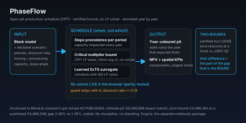
phaseflow pipeline
Technology Stack
In action
A short tour of the live app: the real interface, recorded from the deployed site.

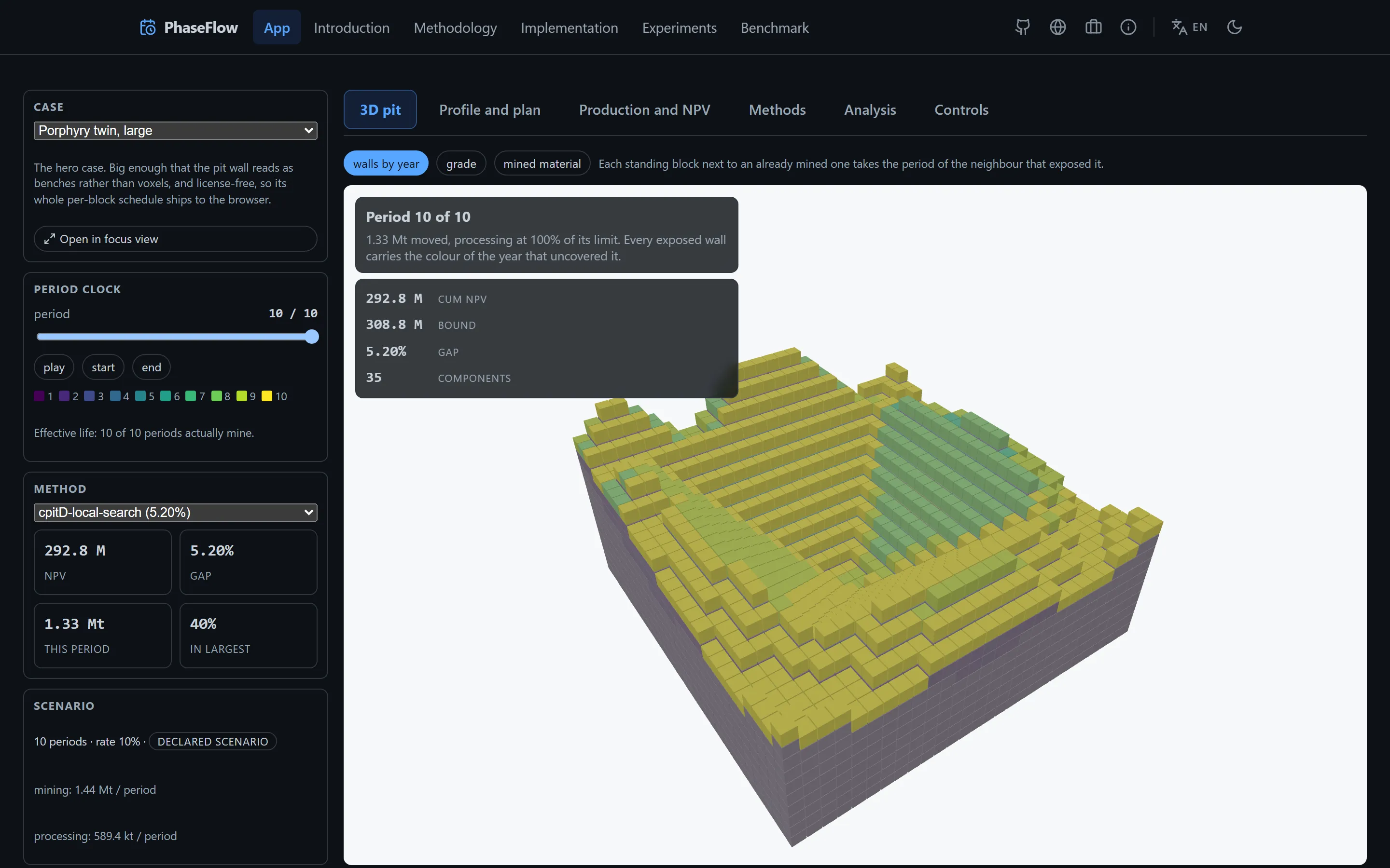
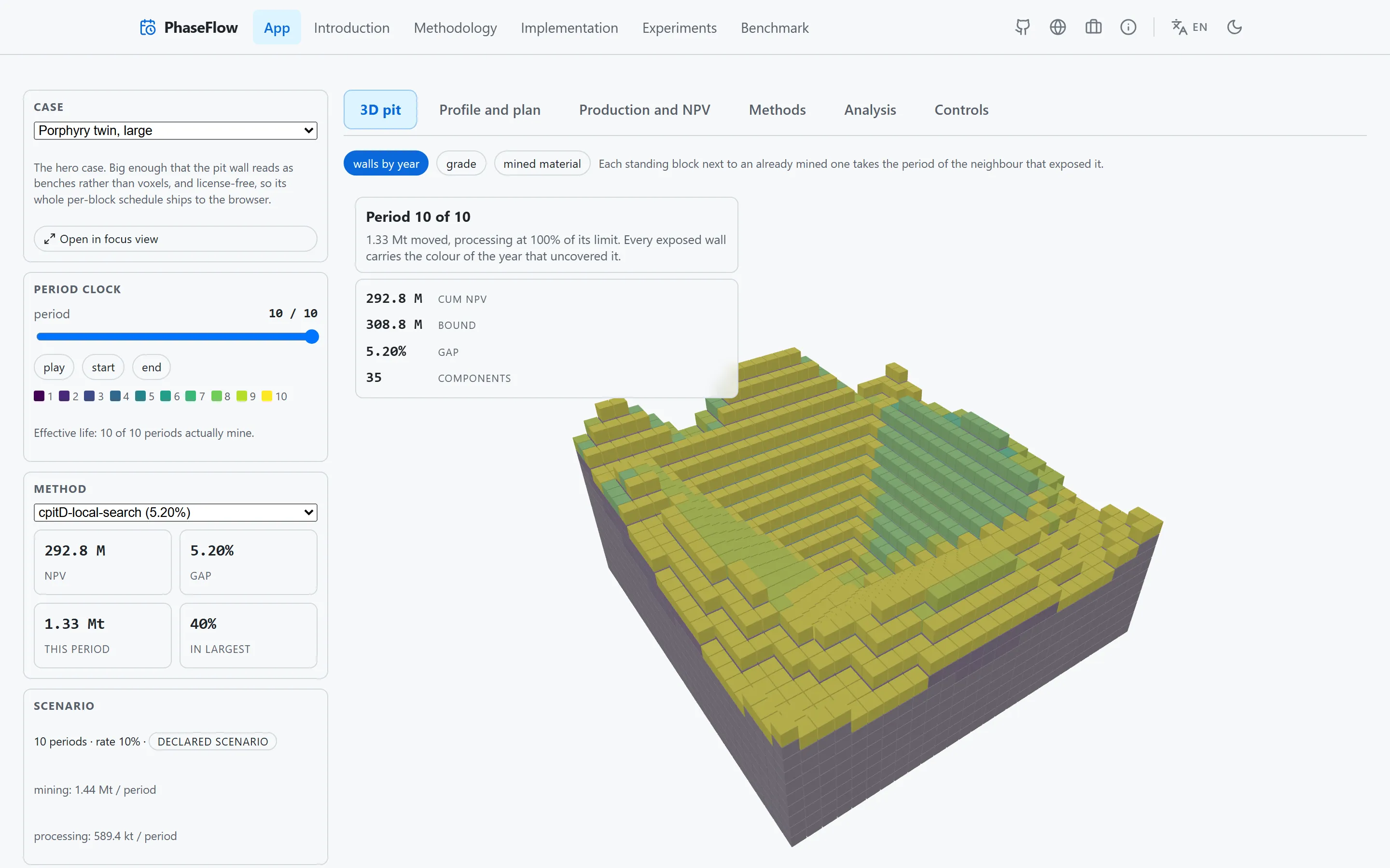
Application Screenshots